

Linear regression is often one of the first algorithms that data analysts are introduced to. The intuition is simple: find the best line that fits a given data set. For example, given the below data set:

you’d probably answer with something along these lines:
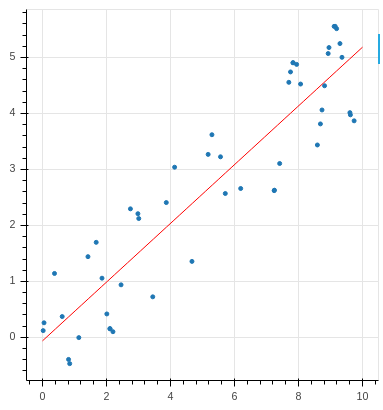
That is, in fact, the answer given by Linear Regression. However, just as the name implies, the algorithm makes a major assumption about your data – that it is linear. The formal equation for linear data is:
y = mx + b
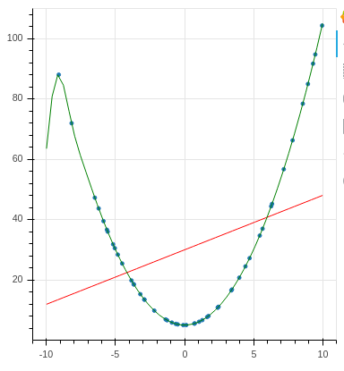
Linear regression assumes that formula is correct and proceeds to find the best fitting values for “m” and “b” the produces the best line going through your data. For some data sets, like the one above – this is a fair approximation. For others, like the one below, not so much…

In the above data set, it’s pretty easy to see that the data is following an x2 formula, rather than a linear one. So our linear assumption doesn’t hold. You could find a regressor that can tackle x2, and repeat
…but wouldn’t it be nice, if we didnt’ have to make any assumptions about the formula at all? Couldn’t we let the regressor find the best function for us?
And that, is exactly what Gaussian Process Regressor does for us. There’s plenty of material on the Internet explaining the theory – so i’ll leave you to it. Intuitively, the Gaussian Process Regressor generates a pool of candidate formulas (in math lingo: “a distribution of functions“) that could have generated the observed data, and attempts to find the best match (in math lingo: Bayesian inference). Then it selects the best candidate and proceeds to use that formula for predicting our data. Applying Gaussian Process Regression to the above data set, we get a much more satisfying:
Gaussian Processes can offer surprising insights into your data
To illustrate this better – remember that original data set we saw before? The “linear” one?
… yeah I lied that’s not quite linear.
Let’s fit a Gaussian process regressor:

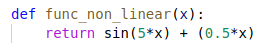
There’s a periodicity in our data set. In fact, the formula to generate the data points actually was:
Show me the code
Gaussian process regression isn’t much harder than Linear Regression to implement. Scikit-learn has this as part of the library. The only difference is the addition of a “kernel” argument. The “kernel” represents your “covariance matrix”. Another math lingo term for a measure of how much “X” depends on “Y”:

The different “kernels” offered by scikit are different covariance matrices. Luckily, the default RBF kernel does a pretty good job in most cases. Other than that, it’s very simple:

A full notebook with code can be found here:
Bonus 1: standard deviation
Gaussian Proccess also allows you to view the standard deviation of a prediction at a certain point. This is useful in visualizing the amount of “uncertainty”. The higher the standard deviation, the lower the certainty. In the code example, the standard dev was very small, so I artificially inflated the standard dev values for easier visualization on the plot by multiplying the real values by a factor of 100:

Bonus 2: can it fit linear data though? (I want a drop in replacement for Linear Regressor)
Yes… with the correct kernel choice.
For example, the green line in the below plot is the Gaussian process regressor estimate for a truly linear dataset (with some random noise added), using the default RBF kernel:

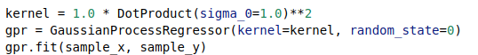
Note how the RBF kernel has too much “freedom” and selects a function with quite a bit of “bends”. Depending on your application, this is probably not the best outcome, so you need a more “rigid” kernel like the “DotProduct” kernel, which gives us something like the following:


You must be logged in to post a comment.