3 uses for random decision trees / forests you (maybe) didn’t know about

Decision tree forests rightly get a lot of attention due to their robust nature, support for high dimensions and easy decipherability. The most well known uses of decision tree forests are:

• Classification – given a set of samples with certain features, classify the samples into discrete classes which the model has been trained on.
• Regression – given a set of samples with certain features, predict a value

However, did you know that Decision Tree Forests also allow you to extract Embeddings?

What are Random Trees Embeddings?

Random Trees embeddings are quite straightforward:

1. Train a random tree forest classifier / regressor as you normally would
2. For any sample you’d like the embedding of, pass the sample through each tree and note which leaf node it ends up in.
3. The leaf node in which the decision tree places the sample is marked as 1, the others are marked as 0
4. Concatenate the vectors together.

As a simple example, consider the following “forest” of 2 trees:

A sample passing through the two trees in the forest ends up with an embedding of [1, 0, 0, 1] due to it’s placement in the trees. Scikit learn provides a ready made function to do all the above:

sklearn.ensemble.RandomTreesEmbedding

If you need more control over the process (for example using an already trained Classifier or Regressor, you can achieve the same affect by using the apply() function.

This gives rise to three interesting use cases:

1. Increasing the dimensionality of your data set
2. Decreasing the dimensionality of your data set
3. Using them to generate a proximity matrix, along with MDS can be used to get better embeddings of high dimension samples

Increasing dimensionality

Even though samples may have a small number of dimensions, the trees themselves may have quite a large number of leaf nodes. As a practical example, imagine the following decision tree on whether to issue a loan:

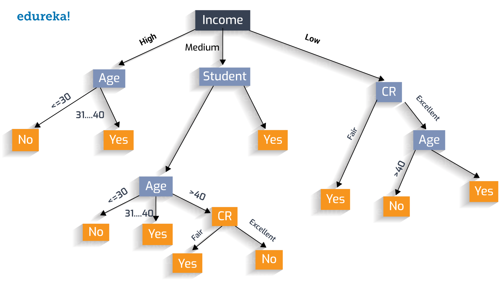
In the above tree, we have 3 features: income, age, and Credit Rating (CR). However, there are 10 terminal nodes (yes/no). Getting an embedding from the above would result in something like [0, 0, 0, 0, 0, 0, 0, 0, 0, 1]. Add to this the fact that a forest can have hundreds of similar trees. and we end up with an embedding that has a large number of dimensions considering we started of with 3.

Why would we want to do this?

In high-dimensional spaces, linear classifiers often achieve excellent accuracy.

Scikit Documentation

This means that Random Forest Embeddings can be an excellent pre-processing step to your linear classification tasks.

Decreasing dimensionality

Of course, this can go the other way. Often, we’re interested in the exact opposite of increasing dimensionality. We typically use techniques like PCA to reduce the number of features that we need to deal with. We can reduce dimensionality of our data set in a couple of ways using decision forests:

1. Modify the decision tree hyper-parameters such as maximum number of leaves (and other similar hyper-parameters) to reduce the number of resulting dimensions from our samples
2. Use decomposition techniques like Truncated SVD on our embeddings
3. Using the resulting “feature importances” to discard unnecessary features, for example on the iris dataset:

Proximity Matrix

A proximity matrix is a related concept to embeddings. The intuition is that similar data points should end up in the same leaf node of a decision tree (taking our first example decision tree above, most high income under 30s will end up in the first “no” terminal node).

So, when comparing two data points, we pass each sample through the forest and note which terminal nodes they end up in for each tree in the forest. If for a given tree in the forest, both samples end up in the same node, then we increase the similarity score by one. Last by not least we normalize the similarity score by dividing the result by the total number of trees in the forest, ending up with a score between 0 (the two samples did not share any common nodes on any trees in the forest), to 1 (the two samples ended up on the same node on all the trees in the forest).

This alone is useful to calculate a “similarity score”. However, we can also repeat this for all samples in the data set and end up with a matrix of size (n_samples x n_samples). This is the proximity matrix. MDS is useful with exactly this type of data to plot the result on a plane – ending up with excellent 2D embeddings