

I’ve recently published the thesis I wrote in fulfillment of my Masters in Computer Security, entitled
BioRFID: A Patient Identification System using Biometrics and RFID
Anyone interested can download and read the whole thesis here:
In this article I’ll give an extremely compressed version of the thesis and how the work therein can be translated to the cybersecurity domain – along with some practical code to illustrate my points.
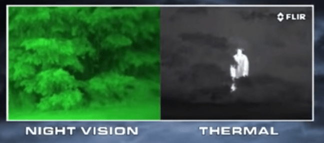
In the physical world, we often translate visual data from one “dimension” to another. For example, looking at the picture below, on the left hand side we see a view using night vision – and we’re still unable to pick out any “anomalies”. The anomaly (standing person) becomes pretty clear when we translate the night google data to use infrared instead, and as can be seen on the right hand side, though we lose some image detail we are now easily able to pick out our “anomaly”
In machine learning, we spend a lot of time trying to find “dimensions” to represent our data in such a way as to make the anomalies we’re looking for stand out far more than if we leave the data in it’s original form. There are a multitude of dimensions we can use, the one presented in the thesis is called “Sparse Coding“. The essence of sparse coding can be explained by examining the figure below:
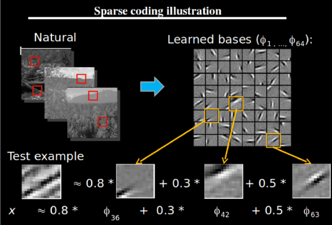
Imagine we have a set of data (images of a forest in the figure above). We can pass this data through a “dictionary learner“. The job of the dictionary learner is to decompose our data into a set of unique “bases” or “atoms“. Just like in the real world, a language dictionary can be used to construct sentences. Any sentence I write can be decomposed into individual words that can subsequently be looked up in a dictionary.
Similarly in our previous example above, any picture can be decomposed into bases or atoms which can be found in the dictionary we just built from our training data. In the specific example in the figure, the bottom “test example” is expressed in terms of three basis, each in different proportions (0.8 for the first one, 0.3 for the second one, and 0.5 for the last one)
Applying this to Cyber Security
Intuitively, such a system will struggle to express data it has never seen before – because it lacks the words or basis to decompose this data. Similarly, unusual or uncommon data will be expressed using a different set of words than those used to express common or normal data. Let’s test this theory.
Take the following practical scenario:
You collect data logs from your firewall, every 5 minutes. Being a good DevOps engineer, you write a quick script to summarize this data, converting all the data in a 5 minute time windows to:
- The destination BGP AS number (because tracking each individual destination IP provides too many entries…)
- The bytes transferred between your network and the destination AS number during those 5 minutes
- The number of clients in your network that communicated with the destination AS number
You would end up with a dataset that looks something like the below. I built the below data set by using LibreOffice calc, randomly generating numbers for each entry. The only difference being the last entry, where I purposely entered an anomalous entry for demo purposes
This file contains hidden or bidirectional Unicode text that may be interpreted or compiled differently than what appears below. To review, open the file in an editor that reveals hidden Unicode characters.
Learn more about bidirectional Unicode characters
| AS Number | Bytes Trans | Clients | |
|---|---|---|---|
| 450 | 644 | 35 | |
| 450 | 429 | 31 | |
| 450 | 677 | 39 | |
| 450 | 299 | 19 | |
| 450 | 792 | 13 | |
| 450 | 318 | 17 | |
| 450 | 544 | 17 | |
| 450 | 679 | 38 | |
| 450 | 418 | 17 | |
| 450 | 798 | 26 | |
| 450 | 220 | 18 | |
| 450 | 151 | 12 | |
| 450 | 796 | 14 | |
| 450 | 744 | 38 | |
| 450 | 523 | 21 | |
| 450 | 571 | 33 | |
| 450 | 278 | 39 | |
| 450 | 123 | 21 | |
| 450 | 654 | 23 | |
| 450 | 380 | 27 | |
| 450 | 350 | 35 | |
| 450 | 785 | 43 | |
| 450 | 549 | 46 | |
| 450 | 357 | 49 | |
| 450 | 621 | 47 | |
| 450 | 146 | 35 | |
| 450 | 273 | 17 | |
| 450 | 510 | 21 | |
| 450 | 595 | 44 | |
| 450 | 139 | 46 | |
| 450 | 716 | 11 | |
| 450 | 689 | 27 | |
| 450 | 756 | 30 | |
| 450 | 662 | 39 | |
| 450 | 448 | 26 | |
| 450 | 738 | 21 | |
| 450 | 512 | 49 | |
| 450 | 401 | 35 | |
| 450 | 404 | 47 | |
| 450 | 188 | 42 | |
| 450 | 479 | 22 | |
| 450 | 729 | 16 | |
| 450 | 767 | 40 | |
| 450 | 542 | 33 | |
| 450 | 483 | 35 | |
| 450 | 361 | 23 | |
| 450 | 541 | 25 | |
| 450 | 234 | 49 | |
| 450 | 780 | 43 | |
| 450 | 656 | 38 | |
| 400 | 651 | 25 | |
| 400 | 521 | 39 | |
| 400 | 353 | 43 | |
| 400 | 145 | 16 | |
| 400 | 714 | 38 | |
| 400 | 640 | 42 | |
| 400 | 265 | 11 | |
| 400 | 552 | 16 | |
| 400 | 369 | 16 | |
| 400 | 729 | 28 | |
| 400 | 249 | 12 | |
| 400 | 752 | 24 | |
| 400 | 134 | 24 | |
| 400 | 545 | 25 | |
| 400 | 364 | 31 | |
| 400 | 547 | 15 | |
| 400 | 318 | 29 | |
| 400 | 713 | 38 | |
| 400 | 273 | 25 | |
| 400 | 104 | 27 | |
| 400 | 725 | 15 | |
| 400 | 738 | 48 | |
| 400 | 410 | 18 | |
| 400 | 234 | 43 | |
| 400 | 639 | 40 | |
| 400 | 235 | 28 | |
| 400 | 690 | 33 | |
| 400 | 324 | 18 | |
| 400 | 336 | 39 | |
| 400 | 565 | 16 | |
| 400 | 787 | 13 | |
| 400 | 399 | 28 | |
| 400 | 301 | 35 | |
| 400 | 201 | 41 | |
| 400 | 634 | 41 | |
| 400 | 693 | 23 | |
| 400 | 518 | 48 | |
| 400 | 221 | 19 | |
| 400 | 573 | 34 | |
| 400 | 599 | 12 | |
| 400 | 758 | 25 | |
| 400 | 595 | 25 | |
| 400 | 227 | 48 | |
| 400 | 745 | 34 | |
| 200 | 149 | 49 | |
| 200 | 163 | 28 | |
| 200 | 129 | 20 | |
| 200 | 128 | 24 | |
| 200 | 88 | 38 | |
| 200 | 143 | 23 | |
| 200 | 161 | 35 | |
| 200 | 125 | 28 | |
| 200 | 147 | 23 | |
| 200 | 160 | 25 | |
| 200 | 101 | 21 | |
| 200 | 186 | 31 | |
| 200 | 96 | 11 | |
| 200 | 131 | 45 | |
| 200 | 99 | 16 | |
| 200 | 171 | 49 | |
| 200 | 92 | 29 | |
| 200 | 167 | 26 | |
| 200 | 121 | 39 | |
| 200 | 159 | 34 | |
| 200 | 174 | 29 | |
| 200 | 135 | 19 | |
| 200 | 107 | 24 | |
| 200 | 80 | 42 | |
| 200 | 166 | 46 | |
| 200 | 164 | 38 | |
| 80 | 1500 | 1 |
Now, you are required to find from within these entries any anomalous or weird data. ideally, you should be able to use your work to calculate if future data points are anomalous or not.
We can apply the sparse coding principles I introduced in this article, as follows – using python, pandas and scipy:
This file contains hidden or bidirectional Unicode text that may be interpreted or compiled differently than what appears below. To review, open the file in an editor that reveals hidden Unicode characters.
Learn more about bidirectional Unicode characters
| from sklearn.decomposition import DictionaryLearning | |
| from sklearn.decomposition import SparseCoder | |
| import pandas as pd | |
| # load data from CSV | |
| df = pd.read_csv('/mnt/c/Users/davev/Documents/test_sparse.csv') | |
| # get rid of the "label" column – AS Number in our case | |
| del df['AS Number'] | |
| # change data into required format from scikit learn | |
| t=df.as_matrix() | |
| # create a dictionary with 2 components (to make it easier to plot later) | |
| # the dictionary is learnt by iterating over the data a 100 times | |
| dict=DictionaryLearning(n_components=2, max_iter=100) | |
| dict.fit(t) | |
| # load the dictionary we just created into a Sparse Coder | |
| sp = SparseCoder(dict.components_) | |
| # instruct the sparse coder to represent our data in terms of the dictionary we previously "learnt" | |
| sp.transform(t) | |
| # … [results displayed] … |
The above code is basically using sparse coding to translate our data from one dimension to another (keep in mind that when doing so we usually can pick out details that are usually hidden, as in our night vision vs infrared example). The resulting data is shown at the end of the article, but it’s easier to visualise the data as a plot, shown below:

We immediately note three anomalies. One translates to the purposely anomalous data point I inserted into the end of our toy data set (as expected), while the other two are anomalies introduced by the random numbers generated. If we examine these further, it turns out that both these anomalies come from AS number “200”, which typically has “number of bytes transferred” being over 100. However for these two cases the number of bytes transferred turned out to be lower than expected – at about 80.
And there you have it – a quick and easy way of detecting anomalous data from firewall logs. Not only that, but you can use the dictionary generated by your code to see if new data points are anomalous or not. Of course this method doesn’t cover all cases and probably has its own set of problems but it’s a very good start considering the minimal amount of work we just put in.
At CyberSift we develop more advanced techniques which leverage machine learning and artificial intelligence to perform anomaly detection as we presented above – but on a much more advanced scale and in a more user friendly manner. Check us out!
Resulting data after sparse coding:
This file contains hidden or bidirectional Unicode text that may be interpreted or compiled differently than what appears below. To review, open the file in an editor that reveals hidden Unicode characters.
Learn more about bidirectional Unicode characters
| Component 1 | Component 2 | |
|---|---|---|
| -644.72435929 | 0 | |
| -429.69628601 | 0 | |
| -677.82285221 | 0 | |
| -299.41280182 | 0 | |
| -792.05515776 | 0 | |
| -318.34981967 | 0 | |
| -544.2623755 | 0 | |
| -679.79426304 | 0 | |
| -418.31112756 | 0 | |
| -798.4144355 | 0 | |
| -220.41555326 | 0 | |
| -151.27535885 | 0 | |
| -796.08142541 | 0 | |
| -744.76911317 | 0 | |
| -523.38176216 | 0 | |
| -571.69697387 | 0 | |
| -278.97723372 | 0 | |
| -123.53653059 | 0 | |
| -654.38670615 | 0 | |
| -380.60398383 | 0 | |
| -350.83811409 | 0 | |
| -785.89232604 | 0 | |
| -550.0670854 | 0 | |
| -358.22482023 | 0 | |
| -622.06704241 | 0 | |
| -146.91704599 | 0 | |
| -273.36723111 | 0 | |
| -510.38679213 | 0 | |
| -595.99365637 | 0 | |
| -140.22572304 | 0 | |
| -716.02893311 | 0 | |
| -689.48442522 | 0 | |
| -756.54194749 | 0 | |
| -662.82865602 | 0 | |
| -448.54985787 | 0 | |
| -738.29857412 | 0 | |
| -513.16484746 | 0 | |
| -401.81838111 | 0 | |
| -405.15100428 | 0 | |
| -189.0955026 | 0 | |
| -479.42660201 | 0 | |
| -729.16297978 | 0 | |
| -767.81584464 | 0 | |
| -542.70819459 | 0 | |
| -483.78665358 | 0 | |
| -361.50007402 | 0 | |
| -541.48605889 | 0 | |
| -235.27241152 | 0 | |
| -780.89426064 | 0 | |
| -656.80316222 | 0 | |
| -651.44349757 | 0 | |
| -521.88321189 | 0 | |
| -354.05947594 | 0 | |
| -145.38894168 | 0 | |
| -714.7807208 | 0 | |
| -640.92061427 | 0 | |
| -265.20343452 | 0 | |
| -552.23146481 | 0 | |
| -369.30227136 | 0 | |
| -729.49676371 | 0 | |
| -249.23744058 | 0 | |
| -752.37660321 | 0 | |
| -134.61572044 | 0 | |
| -545.4845112 | 0 | |
| -364.72143588 | 0 | |
| -547.20558408 | 0 | |
| -318.6836036 | 0 | |
| -713.78110772 | 0 | |
| -273.58975373 | 0 | |
| -104.71077405 | 0 | |
| -725.13671213 | 0 | |
| -739.04958797 | 0 | |
| -410.34203825 | 0 | |
| -235.10551955 | 0 | |
| -639.86537053 | 0 | |
| -235.68790272 | 0 | |
| -690.65093027 | 0 | |
| -324.37531347 | 0 | |
| -336.95479229 | 0 | |
| -565.22643483 | 0 | |
| -787.05709237 | 0 | |
| -399.62444766 | 0 | |
| -301.85707322 | 0 | |
| -202.06265729 | 0 | |
| -634.89512047 | 0 | |
| -693.37161623 | 0 | |
| -519.1347106 | 0 | |
| -221.44298167 | 0 | |
| -573.72401536 | 0 | |
| -599.10201821 | 0 | |
| -758.40209701 | 0 | |
| -595.46516515 | 0 | |
| -228.24730464 | 0 | |
| -745.65746493 | 0 | |
| -150.30529981 | 0 | |
| -163.71576104 | 0 | |
| -129.50639373 | 0 | |
| -128.61804196 | 0 | |
| 0 | -92.10275168 | |
| -143.58442282 | 0 | |
| -161.91124217 | 0 | |
| -125.73046404 | 0 | |
| -147.58287514 | 0 | |
| -160.63347582 | 0 | |
| -101.54504285 | 0 | |
| -186.79030783 | 0 | |
| -96.26882418 | 0 | |
| -132.20100308 | 0 | |
| -99.40674005 | 0 | |
| -172.29678755 | 0 | |
| -92.77104776 | 0 | |
| -167.6585827 | 0 | |
| -122.03798032 | 0 | |
| -159.88420069 | 0 | |
| -174.73932023 | 0 | |
| -135.47625688 | 0 | |
| -107.62616731 | 0 | |
| 0 | -88.46521494 | |
| -167.21527617 | 0 | |
| -164.99352739 | 0 | |
| -1499.44743371 | 0 |

You must be logged in to post a comment.