Analyzing credit card transactions using machine learning techniques – 2

Principal Component Analysis – Introduction and Data Preperation

Principal Component Analysis [PCA] is an unsupervised algorithm which reduces dimensionality and is widely used. A good visual explanation can be found here:

http://setosa.io/ev/principal-component-analysis/

As mentioned in our previous article, Correspondence Analysis  works exclusively on categorical data. In contrast, PCA accepts only numerical data. This means our data set needs to be pre-processed before being fed into PCA. We perform two pre-processing steps:

• We turn the categorical columns into numerical data by using one-hot representation. This creates new columns – each populated with “0” or “1” depending on the original data (see link for more details). This process changes the categorical data into numerical data, at the cost of increasing the number of dimensions (this is not always a good thing – see “the curse of data dimensionality“)
• We normalize the “total” column so that its’ values range between 0 to 1, with 0 being equivalent to the original minimum value and 1 being equivalent to the original maximum value. This makes the “total” column more in line with the other columns which also range between 0 and 1. In turn this makes PCA more accurate

Results

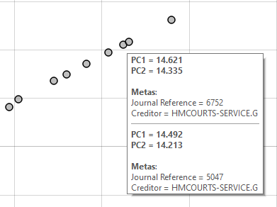
In a similar scenario to what we’ve seen in Correspondence Analysis, most of the observations are grouped in the bottom left corner, with outliers that may represent anomalies trailing off towards the top right. Knowing what we do about our data set, a good guess would be that the relatively linear nature of the anomalies is probably due to the “total” column – which due to it’s numerical nature (as opposed to categorical converted to one-hot representation) has far more variance than the other columns.

Starting with the most obvious top-rightmost outlier:

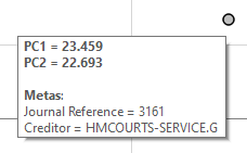
The outlier corresponds to an entry with an extraordinarily large “total” of money transferred, in fact the amount is the maximum number in the data set:

In fact the more pronounced outliers follow the same pattern, all of the observations are payments to the “HMCOURTS-SERVICE“, each of which have abnormally high “total” entries:

The next interesting outlier is a slightly below this linear streak:

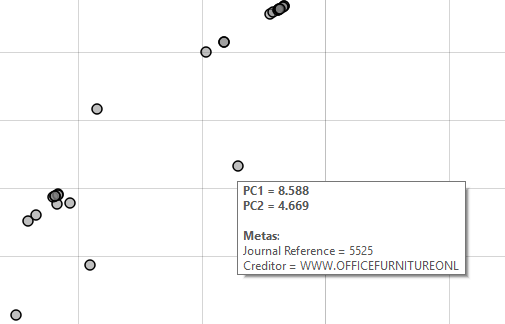
This outlier again corresponds to a rather high “total”, however placed to a different service type (“Furniture-Purchase-Repair“). This would explain why the outlier is on a lower plane than the others.

Conclusions

Compared to correspondence analysis, PCA was more heavily influenced by the “total” column, and hence the results are helpful in identifying outliers which have higher than average “totals”. This is very useful considering this data set is focused around the “total” column – however we would have missed some important relations in the data set had we not also analysed the data using correspondence analysis.

In the next last article of this series we discuss a clustering algorithm which makes it easier to identify outliers in our data without having to manually process the results of PCA as we did above

Analyzing credit card transactions using machine learning techniques – 1
Analyzing credit card transactions using machine learning techniques – 3