

Scenario: Measuring the number of HTTP response codes returned to clients over time using InfluxDB. This would (for example) produce a line graph with a line for each HTTP code (e.g. 200, 500, 404, etc) which varies over time
We use InfluxDB (latest version is 2.0.8 at the time of writing) to monitor much of our services, including those of our new Tutela service. Part of the Tutela infrastructure is an NGINX reverse proxy which performs several routing and load-balancing operations, so it’s an important piece of the tech stack to monitor.
InfluxDB already has an in-built Telegraf input plugin to monitor NGINX which depends on the NGINX stub-status module:
https://github.com/influxdata/telegraf/tree/master/plugins/inputs/nginx
That works great and does give you a good indication of NGINX activity, for example:

However, note how there are only two “lines”… for active and waiting connections respectively. What if we’d like to further subdivide this graph into returned HTTP response codes (200, 500, 404 etc) to give NOC a better idea of what is going on? To do this, we need to use a different approach which turns out to be instructive both in terms of using a different Telegraf input plugin and using the InfluxDB Flux query language
Note: the following methodology should work for both Apache and Nginx servers, though we keep our focus on Nginx here
TLDR: use the “file” input plugin and a custom InfluxDB flux query to show the appropriate graph
Step 1: Install Telegraf on the webserver and configure the “file” input plugin
Our method is going to depend in shipping the server access logs back to the InfluxDB instance. This is very straightforward using the “tail” telegraf input plugin:
[[inputs.tail]]
  ## Files to parse each interval.
  ## These accept standard unix glob matching rules, but with the addition of
  ## ** as a "super asterisk". ie:
  ##   /var/log/**.log     -> recursively find all .log files in /var/log
  ##   /var/log/*/*.log    -> find all .log files with a parent dir in /var/log
  ##   /var/log/apache.log -> only tail the apache log file
  files = ["/var/log/nginx/access.log"]

  ## The dataformat to be read from files
  ## Each data format has its own unique set of configuration options, read
  ## more about them here:
  ## https://github.com/influxdata/telegraf/blob/master/docs/DATA_FORMATS_INPUT.md
  data_format = "grok"

  ## This is a list of patterns to check the given log file(s) for.
  ## Note that adding patterns here increases processing time. The most
  ## efficient configuration is to have one pattern.
  ## Other common built-in patterns are:
  ##   %{COMMON_LOG_FORMAT}   (plain apache & nginx access logs)
  grok_patterns = ["%{COMBINED_LOG_FORMAT}"]
The config above is what we used in is very well commented by the InfluxDB team, the important thing to note is that we use the “grok” data format and we set the grok pattern to COMBINED_LOG_FORMAT, which is what NGINX is set to use by default
Step 2: Query the data being sent to InfluxDB
Here we’l use the “Data Explorer” tab and set it to use the “script editor” and “view raw data” as shown below:

Sidenote: I’d advise to take this step by step and view the results returned from your query at every stage so you’ll understand what’s going on
Our first step is to pull data from the appropriate bucket, within our required timeframe and from the “tail” plugin:
from(bucket: "YOUR_BUCKET_HERE")
  |> range(start: v.timeRangeStart, stop: v.timeRangeStop)
  |> filter(fn: (r) => r["_measurement"] == "tail")
So far it’s quite standard, we use from() to pull from the appropriate bucket, range() to set the timeframe and filter() to filter for those records which have the “_measurement” key set to “tail”. _measurement is a reserved key which telegraf uses to mark which input plugin produced the record, and in our case this is set to “tail” since we used the tail plugin.
If you peer at the resulting table, you’ll see something like:

Note in particular that first line starting with “#group” which is set to true or false for each column. The group is currently set to true for the following columns:
- _field
- _measurement
- host
- path
- resp_code
- verb
Grouping means a new table will be created for any new combination of the above fields. In fact scrolling down the results you’ll notice the the “table” column increments in number if you do in fact have a different combination of the above.
Each table will be producing a separate line in the graph, so we’re not quite where we want to be. We’d like to have a graph line for each resp_code ONLY, not each verb, host, and path too. So our next part of the query will be to change this behavior and limit our grouping to just the resp_code:
from(bucket: "YOUR_BUCKET_HERE")
  |> range(start: v.timeRangeStart, stop: v.timeRangeStop)
  |> filter(fn: (r) => r["_measurement"] == "tail")
  |> group(columns: ["resp_code"], mode:"by")
That’s what the group() function does, and after running the above you’ll note that the “#group” line in the results table now shows “true” only for resp_code.
We’re almost there… but notice how if you scroll through the results table, you’ll see the key “_field” changing to elements from the log like “agent”, “client_ip” and so on. This will results in erroneous counts since each log line from tail is split into multiple rows in the table, each with a different “_field”. So we need to focus on just one _field. We picked “client_ip” but this can be any field which appears in all log lines:
from(bucket: "YOUR_BUCKET_HERE")
  |> range(start: v.timeRangeStart, stop: v.timeRangeStop)
  |> filter(fn: (r) => r["_measurement"] == "tail")
  |> filter(fn: (r) => r["_field"] == "client_ip")
  |> group(columns: ["resp_code"], mode:"by")
Note that we inserted the new line right before our group() function to ensure proper filtering. The last step is to aggregate our results into time windows which can be plotted on the graph, which is exactly what the aggregateWindow() function does:
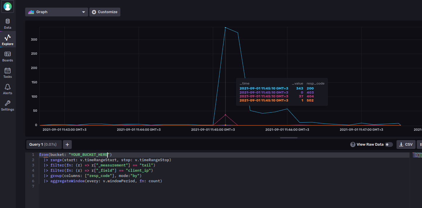
from(bucket: "YOUR_BUCKET_HERE")
  |> range(start: v.timeRangeStart, stop: v.timeRangeStop)
  |> filter(fn: (r) => r["_measurement"] == "tail")
  |> filter(fn: (r) => r["_field"] == "client_ip")
  |> group(columns: ["resp_code"], mode:"by")
  |> aggregateWindow(every: v.windowPeriod, fn: count)
Of special note is the use of the count() function to be used by aggregateWindow, so that we make sure the aggregation is counting the number of log entries within the given time window.
If you now remove the “View Raw Data” switch, you’ll see the appropriate graph being plotted:

You must be logged in to post a comment.